ここにメモを残していく（自分用）。

分析手法

階層的重回帰分析

　階層的重回帰分析は、ステップ１からステップ２へとステップごとに関心のある変数を投入していき、分散説明率が統計的に有意に増加することを検定することで、その変数の重要性を分析する手法である。
　たとえば、大事な人に会うときや人前で話をするとき、誰しも不安を感じやすい（状態不安という）。そのときの不安の程度は、協調性や誠実さといったパーソナリティ特性によることが考えられるが、研究として関心があるのはこれらの交互作用効果だとする（“誠実さが高く協調性が高い人は周囲に合わせようとするため、不安を感じやすい”とか）。その場合は、ステップ１では説明変数として“協調性”と“誠実さ”を入れ、ステップ２ではさらに“協調性”と“誠実さ”の交互作用項を入れて分析する。ただし、各変数と交互作用項の相関による多重共線性の問題が考えられるので中心化処理（平均値を引く）を忘れずに行う。

分析

　Rで分析する場合には以下のコードを用いる。
　

data <- XXX  #<U+5206><U+6790><U+3057><U+305F><U+3044><U+30C7><U+30FC><U+30BF><U+3092><U+5165><U+308C><U+308B>
y <- data$v1  #<U+5FDC><U+7B54><U+5909><U+6570>: <U+72B6><U+614B><U+4E0D><U+5B89>
x1 <- data$v2 - mean(data$v2)  #<U+8AAC><U+660E><U+5909><U+6570>(<U+4E2D><U+5FC3><U+5316>): <U+5354><U+8ABF><U+6027>
x2 <- data$v3 - mean(data$v3)  #<U+8AAC><U+660E><U+5909><U+6570>(<U+4E2D><U+5FC3><U+5316>): <U+8AA0><U+5B9F><U+3055>
c1 <- data$v4 - mean(data$v4)  #<U+5171><U+5909><U+91CF>(<U+4E2D><U+5FC3><U+5316>): <U+795E><U+7D4C><U+75C7><U+50BE><U+5411>

# <U+7B2C>1<U+30B9><U+30C6><U+30C3><U+30D7>
step1 <- lm(y ~ x1 + x2 + c1)
summary(step1)

# <U+7B2C>2<U+30B9><U+30C6><U+30C3><U+30D7>
step2 <- lm(y ~ x1 + x2 + x1:x2 + c1)
summary(step2)

# <U+5E73><U+65B9><U+548C><U+306E><U+5909><U+5316><U+91CF><U+306E><U+691C><U+5B9A>
anova(step1, step2)

　　今回は、データセットとしてpsychパッケージに入っている“epi.bfi”を使用する。このデータセットにはアイゼンク性格検査（EPI）とBig 5尺度、ベック抑うつ性尺度、特性‐状態不安の得点が231人分入っている。
　　実際に分析を行う際には、説明変数の数や共変量の有無は適宜調整する。

library(psych)

## 
## Attaching package: 'psych'

## The following objects are masked from 'package:ggplot2':
## 
##     %+%, alpha

data <- epi.bfi  #<U+5206><U+6790><U+3057><U+305F><U+3044><U+30C7><U+30FC><U+30BF><U+3092><U+5165><U+308C><U+308B>
y <- data$stateanx  #<U+5FDC><U+7B54><U+5909><U+6570>: <U+72B6><U+614B><U+4E0D><U+5B89>
x1 <- data$bfcon - mean(data$bfcon)  #<U+8AAC><U+660E><U+5909><U+6570>(<U+4E2D><U+5FC3><U+5316>): <U+5354><U+8ABF><U+6027>
x2 <- data$bfagree - mean(data$bfagree)  #<U+8AAC><U+660E><U+5909><U+6570>(<U+4E2D><U+5FC3><U+5316>): <U+8AA0><U+5B9F><U+3055>
c1 <- data$bfneur - mean(data$bfneur)  #<U+5171><U+5909><U+91CF>(<U+4E2D><U+5FC3><U+5316>): <U+795E><U+7D4C><U+75C7><U+50BE><U+5411>

第1ステップ

step1 <- lm(y ~ x1 + x2 + c1)
summary(step1)

## 
## Call:
## lm(formula = y ~ x1 + x2 + c1)
## 
## Residuals:
##     Min      1Q  Median      3Q     Max 
## -20.622  -6.996  -1.325   5.394  28.091 
## 
## Coefficients:
##             Estimate Std. Error t value Pr(>|t|)    
## (Intercept) 39.84848    0.64525  61.757  < 2e-16 ***
## x1          -0.05379    0.03318  -1.621   0.1064    
## x2          -0.08006    0.04001  -2.001   0.0466 *  
## c1           0.24162    0.02781   8.688  7.4e-16 ***
## ---
## Signif. codes:  0 '***' 0.001 '**' 0.01 '*' 0.05 '.' 0.1 ' ' 1
## 
## Residual standard error: 9.807 on 227 degrees of freedom
## Multiple R-squared:  0.2803, Adjusted R-squared:  0.2708 
## F-statistic: 29.47 on 3 and 227 DF,  p-value: 3.963e-16

第2ステップ

step2 <- lm(y ~ x1 + x2 + x1:x2 + c1)
summary(step2)

## 
## Call:
## lm(formula = y ~ x1 + x2 + x1:x2 + c1)
## 
## Residuals:
##     Min      1Q  Median      3Q     Max 
## -20.660  -6.979  -1.415   5.140  28.356 
## 
## Coefficients:
##              Estimate Std. Error t value Pr(>|t|)    
## (Intercept) 39.330808   0.690941  56.924  < 2e-16 ***
## x1          -0.056617   0.032994  -1.716   0.0875 .  
## x2          -0.083492   0.039784  -2.099   0.0370 *  
## c1           0.234168   0.027875   8.401 4.94e-15 ***
## x1:x2        0.002911   0.001451   2.007   0.0460 *  
## ---
## Signif. codes:  0 '***' 0.001 '**' 0.01 '*' 0.05 '.' 0.1 ' ' 1
## 
## Residual standard error: 9.742 on 226 degrees of freedom
## Multiple R-squared:  0.2929, Adjusted R-squared:  0.2804 
## F-statistic:  23.4 on 4 and 226 DF,  p-value: 3.352e-16

平方和の変化量の検定

anova(step1, step2)

Res.Df	RSS	Df	Sum of Sq	F	Pr(>F)
227	21831.76	NA	NA	NA	NA
226	21449.49	1	382.2643	4.027681	0.0459507

結果の書き方の例

　状態不安得点を応答変数とした階層的重回帰分析を行った。その結果、ステップ1（R²adj = .27, F (3,227) = 29.47, p < .05）から交互作用項を含んだステップ2（R²adj = .28, F (4,226) = 23.40, p < .05）で分散説明率の有意な増加が見られた（ΔR² = .07, ΔF (1,226) = 4.03, p < .05）。誠実さ得点と協調性得点の交互作用効果が有意であった（b* = 0.002, t (226) = 2.01, p < .05）。誠実さ得点の主効果（b* = -0.06, t (226) = 1.72, ns.）は有意ではなかった。協調性得点の主効果が有意であった（b* = -0.08, t (226) = 2.10, p < .05）。共変量の神経症傾向得点の主効果が有意であった（b* = 0.23, t (226) = 8.40, p < .05）。

単純傾斜分析

　交互作用効果が有意であった場合、下位検定として単純傾斜分析を行う。
　コードは以下の通り。　　

# <U+4E0B><U+4F4D><U+691C><U+5B9A>
# x1<U+304C>+1SD<U+306E><U+5834><U+5408><U+306E>x2<U+306E><U+52B9><U+679C><U+3092><U+5206><U+6790>
x1high <- data$v2 - (mean(data$v2) + sd(data$v2))
simpleslope1 <- lm(y ~ x1high + x2 + x1high:x2 + c1)
summary(simpleslope1)

## x1<U+304C>-1SD<U+306E><U+5834><U+5408><U+306E>x2<U+306E><U+52B9><U+679C><U+3092><U+5206><U+6790>
x1low <- data$v2 - (mean(data$v2) - sd(data$v2))
simpleslope2 <- lm(y ~ x1low + x2 + x1low:x2 + c1)
summary(simpleslope2)

x1が+1SDの場合のx2の効果を分析

x1high <- data$bfcon - (mean(data$bfcon) + sd(data$bfcon))
simpleslope1 <- lm(y ~ x1high + x2 + x1high:x2 + c1)
summary(simpleslope1)

## 
## Call:
## lm(formula = y ~ x1high + x2 + x1high:x2 + c1)
## 
## Residuals:
##     Min      1Q  Median      3Q     Max 
## -20.660  -6.979  -1.415   5.140  28.356 
## 
## Coefficients:
##              Estimate Std. Error t value Pr(>|t|)    
## (Intercept) 38.092154   1.007153  37.822  < 2e-16 ***
## x1high      -0.056617   0.032994  -1.716   0.0875 .  
## x2          -0.019799   0.049815  -0.397   0.6914    
## c1           0.234168   0.027875   8.401 4.94e-15 ***
## x1high:x2    0.002911   0.001451   2.007   0.0460 *  
## ---
## Signif. codes:  0 '***' 0.001 '**' 0.01 '*' 0.05 '.' 0.1 ' ' 1
## 
## Residual standard error: 9.742 on 226 degrees of freedom
## Multiple R-squared:  0.2929, Adjusted R-squared:  0.2804 
## F-statistic:  23.4 on 4 and 226 DF,  p-value: 3.352e-16

x1が-1SDの場合のx2の効果を分析

x1low <- data$bfcon - (mean(data$bfcon) - sd(data$bfcon))
simpleslope2 <- lm(y ~ x1low + x2 + x1low:x2 + c1)
summary(simpleslope2)

## 
## Call:
## lm(formula = y ~ x1low + x2 + x1low:x2 + c1)
## 
## Residuals:
##     Min      1Q  Median      3Q     Max 
## -20.660  -6.979  -1.415   5.140  28.356 
## 
## Coefficients:
##              Estimate Std. Error t value Pr(>|t|)    
## (Intercept) 40.569461   0.991228  40.929  < 2e-16 ***
## x1low       -0.056617   0.032994  -1.716  0.08754 .  
## x2          -0.147186   0.051948  -2.833  0.00502 ** 
## c1           0.234168   0.027875   8.401 4.94e-15 ***
## x1low:x2     0.002911   0.001451   2.007  0.04595 *  
## ---
## Signif. codes:  0 '***' 0.001 '**' 0.01 '*' 0.05 '.' 0.1 ' ' 1
## 
## Residual standard error: 9.742 on 226 degrees of freedom
## Multiple R-squared:  0.2929, Adjusted R-squared:  0.2804 
## F-statistic:  23.4 on 4 and 226 DF,  p-value: 3.352e-16

結果の書き方の例

　誠実さ得点と協調性得点の交互作用効果が有意であったため、下位検定として単純傾斜分析を行った。その結果、誠実さ得点を-1SDとした場合、協調性得点の負の効果が確認された（b* = -0.15, t (226) = 2.833, p < .05）。誠実さ得点を+1SDとした場合、協調性得点の有意な効果は認められなかった（b* = -0.02, t (226) = 0.40, ns.）。

　あらら、なんだか変な結果に・・・

探索的因子分析

　科学において測定は重要である。心理学においては、目に見えない心の働きを研究するうえで様々な質問項目が利用されてきており、それがお家芸にもなっている。複数からなる質問項目がいったいどのような概念を表しているのかは関心の高いところであるが、探索的因子分析は項目への回答に影響した因子の存在を統計的に抽出する手法である。

　Rで分析する場合には以下のコードを用いる。

data <- XXX  #<U+5206><U+6790><U+3057><U+305F><U+3044><U+30C7><U+30FC><U+30BF><U+3092><U+5165><U+308C><U+308B>

library(psych)  #psych<U+30D1><U+30C3><U+30B1><U+30FC><U+30B8><U+3092><U+4F7F><U+3046>

# <U+56E0><U+5B50><U+6570><U+306E><U+6C7A><U+5B9A>
va <- data.frame(data$Q1, data$Q2, data$Q3, data$Q4, data$Q5, data$Q6, data$Q7, data$Q8, 
    data$Q9, data$Q10, data$Q11)  #<U+56E0><U+5B50><U+5206><U+6790><U+306B><U+304B><U+3051><U+308B><U+5909><U+6570><U+3092><U+53D6><U+308A><U+51FA><U+3059>

fa.parallel(va)  #<U+63A8><U+5B9A><U+3055><U+308C><U+308B><U+6700><U+5927><U+306E><U+56E0><U+5B50><U+6570>(<U+5E73><U+884C><U+5206><U+6790>)
VSS(va, plot = FALSE)  #<U+63A8><U+5B9A><U+3055><U+308C><U+308B><U+6700><U+5C0F><U+306E><U+56E0><U+5B50><U+6570>(<U+6700><U+5C0F><U+5E73><U+5747><U+504F><U+76F8><U+95A2>)


# <U+63A2><U+7D22><U+7684><U+56E0><U+5B50><U+5206><U+6790>
fa.result <- fa(va, nfactors = 4, fm = "minres", rotate = "promax")  #<U+305F><U+3068><U+3048><U+3070><U+56E0><U+5B50><U+6570><U+3092>4<U+3068><U+3057><U+3066><U+3001><U+6700><U+5C0F><U+4E8C><U+4E57><U+6CD5><U+306E><U+30D7><U+30ED><U+30DE><U+30C3><U+30AF><U+30B9><U+3001><U+3069><U+30FC><U+3093>!
print(fa.result, sort = T, digit = 3, cut = 0.3)  #<U+7D50><U+679C><U+306E><U+8868><U+793A><U+3002><U+30BD><U+30FC><U+30C8><U+304B><U+3051><U+3066><U+3001><U+6841><U+6570><U+306F>3<U+3001>0.3<U+4EE5><U+4E0B><U+306E><U+7D50><U+679C><U+306F><U+30AB><U+30C3><U+30C8>

　上のコードでは、回転法はプロマックス回転、初期解の算出には最小二乗法を用いている。
　回転法（rotate=）については直交回転と斜交回転を選択できる。直交回転なら“varimax”、斜交回転なら“promax”が使えるが、その他の回転法も直交回転と斜交回転のそれぞれ用意されている。
　初期解の算出（fm=）には、最小二乗法なら“minres”、最尤法なら“ml”、主因子法なら“pa”が使える。他にもあり。

因子数の選定

　　因子分析をするにあたってはまず因子数の選定が必要になってくる。基本的には理論的な説明が可能であることが大切だろうが、統計的な算出方法もある。有名なのはスクリープロットでかくんとなってるところを基準に見るやつ。
　その他、平行分析と最小平均偏相関という手法がある（どちらもpsychoパッケージに入ってる）。数学的なことはわからないけど、平行分析は因子数として選定され得る数を大きめに出す。一方、最小平均偏相関は因子数を倹約的に推定する。そのため、因子数はだいたい最小平均偏相関の値から平行分析の値までの間で分析していって、理論的な説明や因子分析のモデル適合度を見ながら最終的な因子数を決めるのが良さそう。
　　データセットとしてpsychパッケージに入っている“epi.bfi”を使用する。このデータセットにはアイゼンク性格検査（EPI）とBig 5尺度、ベック抑うつ性尺度、特性‐状態不安の得点が231人分入っている。

library(psych)  #psych<U+30D1><U+30C3><U+30B1><U+30FC><U+30B8><U+3092><U+4F7F><U+3046>

va <- epi.bfi  #<U+56E0><U+5B50><U+5206><U+6790><U+306B><U+304B><U+3051><U+308B><U+5909><U+6570><U+3092><U+53D6><U+308A><U+51FA><U+3059><U+3002><U+3053><U+3053><U+3067><U+306F><U+3059><U+3079><U+3066><U+306E><U+5909><U+6570><U+3092><U+4F7F><U+3046><U+3002>

平行分析

fa.parallel(va)  #<U+63A8><U+5B9A><U+3055><U+308C><U+308B><U+6700><U+5927><U+306E><U+56E0><U+5B50><U+6570>(<U+5E73><U+884C><U+5206><U+6790>)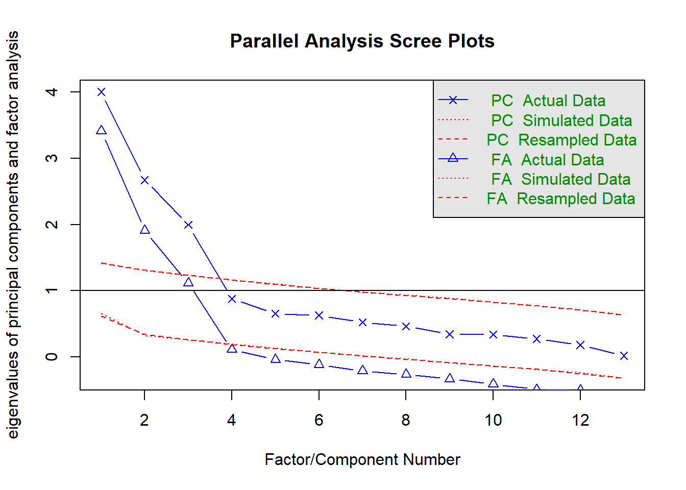

## Parallel analysis suggests that the number of factors =  3  and the number of components =  3

最小平均偏相関

　“The Velicer MAP achieves a minimum of 0.05 with…”のところのfactorsを見る。　　

VSS(va, plot = FALSE)  #<U+63A8><U+5B9A><U+3055><U+308C><U+308B><U+6700><U+5C0F><U+306E><U+56E0><U+5B50><U+6570>(<U+6700><U+5C0F><U+5E73><U+5747><U+504F><U+76F8><U+95A2>)

## 
## Very Simple Structure
## Call: vss(x = x, n = n, rotate = rotate, diagonal = diagonal, fm = fm, 
##     n.obs = n.obs, plot = plot, title = title, use = use, cor = cor)
## VSS complexity 1 achieves a maximimum of 0.73  with  3  factors
## VSS complexity 2 achieves a maximimum of 0.86  with  3  factors
## 
## The Velicer MAP achieves a minimum of 0.05  with  3  factors 
## BIC achieves a minimum of  -22.79  with  6  factors
## Sample Size adjusted BIC achieves a minimum of  -3.74  with  8  factors
## 
## Statistics by number of factors 
##   vss1 vss2   map dof   chisq     prob sqresid  fit RMSEA BIC  SABIC complex
## 1 0.53 0.00 0.098  65 1253.38 2.0e-219    14.0 0.53 0.286 900 1105.6     1.0
## 2 0.70 0.76 0.076  53  704.54 1.2e-114     7.0 0.76 0.235 416  584.1     1.1
## 3 0.73 0.86 0.050  42  354.38  4.8e-51     3.1 0.90 0.183 126  258.9     1.3
## 4 0.71 0.86 0.065  32  262.74  4.6e-38     2.5 0.92 0.181  89  190.0     1.5
## 5 0.65 0.84 0.088  23  142.11  3.8e-19     2.1 0.93 0.153  17   89.8     1.7
## 6 0.63 0.85 0.116  15   58.85  4.0e-07     1.8 0.94 0.116 -23   24.8     1.7
## 7 0.66 0.83 0.147   8   21.71  5.5e-03     1.7 0.94 0.089 -22    3.5     1.8
## 8 0.65 0.81 0.218   2    0.81  6.7e-01     1.3 0.96 0.000 -10   -3.7     1.7
##    eChisq    SRMR eCRMS eBIC
## 1 1.5e+03 0.20267 0.222 1126
## 2 4.9e+02 0.11719 0.142  206
## 3 5.6e+01 0.03932 0.054 -173
## 4 2.8e+01 0.02811 0.044 -146
## 5 1.4e+01 0.01940 0.036 -112
## 6 3.3e+00 0.00952 0.022  -78
## 7 7.7e-01 0.00461 0.014  -43
## 8 1.5e-02 0.00065 0.004  -11

探索的因子分析

　因子数は３因子が良さそう。

fa.result <- fa(va, nfactors = 3, fm = "minres", rotate = "promax")  #<U+56E0><U+5B50><U+6570><U+3092>3<U+3068><U+3057><U+3066><U+3001><U+6700><U+5C0F><U+4E8C><U+4E57><U+6CD5><U+306E><U+30D7><U+30ED><U+30DE><U+30C3><U+30AF><U+30B9><U+3001><U+3069><U+30FC><U+3093>!
print(fa.result, sort = T, digit = 3, cut = 0.3)  #<U+7D50><U+679C><U+306E><U+8868><U+793A><U+3002><U+30BD><U+30FC><U+30C8><U+304B><U+3051><U+3066><U+3001><U+6841><U+6570><U+306F>3<U+3001>0.3<U+4EE5><U+4E0B><U+306E><U+7D50><U+679C><U+306F><U+30AB><U+30C3><U+30C8>

## Factor Analysis using method =  minres
## Call: fa(r = va, nfactors = 3, rotate = "promax", fm = "minres")
## 
##  Warning: A Heywood case was detected. 
## Standardized loadings (pattern matrix) based upon correlation matrix
##          item    MR1    MR2    MR3    h2      u2  com
## epiNeur     5  0.828               0.663  0.3371 1.05
## traitanx   12  0.825               0.821  0.1793 1.15
## bfneur      9  0.821         0.334 0.643  0.3566 1.33
## bdi        11  0.718               0.534  0.4663 1.01
## stateanx   13  0.662               0.451  0.5487 1.01
## epilie      4                      0.187  0.8125 2.39
## epiE        1         1.015        1.050 -0.0497 1.02
## epiImp      3         0.757        0.568  0.4319 1.07
## epiS        2         0.702        0.584  0.4165 1.20
## bfagree     6                0.646 0.449  0.5512 1.03
## bfopen     10                0.642 0.404  0.5963 1.23
## bfcon       7                0.639 0.464  0.5359 1.35
## bfext       8         0.481  0.613 0.685  0.3155 1.90
## 
##                         MR1   MR2   MR3
## SS loadings           3.127 2.541 1.834
## Proportion Var        0.241 0.195 0.141
## Cumulative Var        0.241 0.436 0.577
## Proportion Explained  0.417 0.339 0.244
## Cumulative Proportion 0.417 0.756 1.000
## 
##  With factor correlations of 
##        MR1    MR2    MR3
## MR1  1.000 -0.010 -0.257
## MR2 -0.010  1.000  0.117
## MR3 -0.257  0.117  1.000
## 
## Mean item complexity =  1.3
## Test of the hypothesis that 3 factors are sufficient.
## 
## The degrees of freedom for the null model are  78  and the objective function was  8.247 with Chi Square of  1854.125
## The degrees of freedom for the model are 42  and the objective function was  1.59 
## 
## The root mean square of the residuals (RMSR) is  0.039 
## The df corrected root mean square of the residuals is  0.054 
## 
## The harmonic number of observations is  231 with the empirical chi square  55.713  with prob <  0.0764 
## The total number of observations was  231  with Likelihood Chi Square =  354.378  with prob <  4.81e-51 
## 
## Tucker Lewis Index of factoring reliability =  0.6703
## RMSEA index =  0.1831  and the 90 % confidence intervals are  0.1628 0.1973
## BIC =  125.797
## Fit based upon off diagonal values = 0.985

クラスタ分析

　以下のコードを使う。　

clust <- XXX  #<U+5206><U+6790><U+3057><U+305F><U+3044><U+30C7><U+30FC><U+30BF><U+3092><U+5165><U+308C><U+308B>

# <U+8DDD><U+96E2><U+306E><U+8A08><U+7B97>
uclust <- dist(clust)^2  #<U+30E6><U+30FC><U+30AF><U+30EA><U+30C3><U+30C9><U+8DDD><U+96E2><U+306E><U+5E73><U+65B9>

result <- hclust(uclust, method = "ward.D2")  #Ward<U+6CD5>

groups <- cutree(result, k = 4)  #<U+30AF><U+30E9><U+30B9><U+30BF><U+6570><U+3092>4<U+3064><U+3068><U+3059><U+308B>
groups <- factor(groups)

# <U+30AF><U+30E9><U+30B9><U+30BF><U+306B><U+540D><U+524D><U+3092><U+4ED8><U+3051><U+308B>
levels(groups)[1] <- "Group1"
levels(groups)[2] <- "Group2"
levels(groups)[3] <- "Group3"
levels(groups)[3] <- "Group4"

table(groups)

clust$groups <- groups
aggregate(. ~ groups, data = clust, FUN = mean)

クラスタ数の分析

　クラスタ数を選定する方法として、The Calinski-Harabasz indexがある。
　クラスター数ごとに、クラスタ内の距離の2乗の合計値（within sum of squares; WSS）を算出し、その曲線のエルボーを探す。クラスタ数が増加すると、total WSSが減少するのだが、理想的なクラスター数を超えるとWSSの減少割合が落ちるという見込みからエルボー探しをする。
　また、Calinski-Harabasz基準とは、WSSに対するクラスター間の分散（データセットの重心からすべてのクラスターの重心の分散）の割合である。

library(psych)
clust<-epi.bfi[,6:10]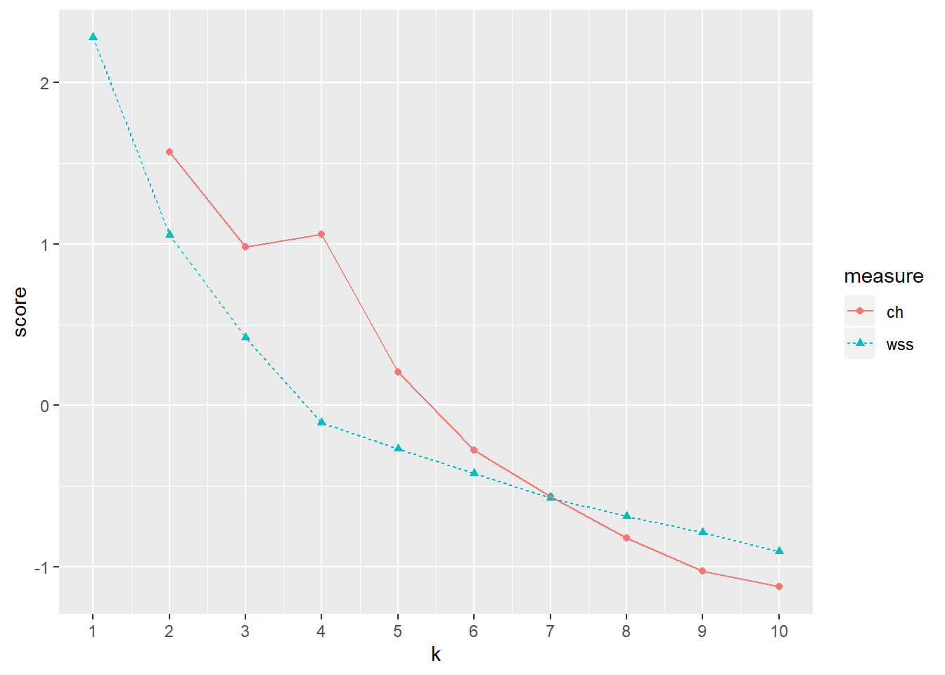

　エルボー…４…かな？

クラスタ分析

# <U+8DDD><U+96E2><U+306E><U+8A08><U+7B97>
uclust <- dist(clust)^2  #<U+30E6><U+30FC><U+30AF><U+30EA><U+30C3><U+30C9><U+8DDD><U+96E2><U+306E><U+5E73><U+65B9>

result <- hclust(uclust, method = "ward.D2")  #Ward<U+6CD5>

groups <- cutree(result, k = 4)  #<U+30AF><U+30E9><U+30B9><U+30BF><U+6570><U+3092>4<U+3064><U+3068><U+3059><U+308B>
groups <- factor(groups)

# <U+30AF><U+30E9><U+30B9><U+30BF><U+306B><U+540D><U+524D><U+3092><U+4ED8><U+3051><U+308B>
levels(groups)[1] <- "Group1"
levels(groups)[2] <- "Group2"
levels(groups)[3] <- "Group3"
levels(groups)[4] <- "Group4"

table(groups)

## groups
## Group1 Group2 Group3 Group4 
##     71     67     35     58

clust$groups <- groups
per <- aggregate(. ~ groups, data = clust, FUN = mean)
per

groups	bfagree	bfcon	bfext	bfneur	bfopen
Group1	126.1408	116.29577	106.46479	62.95775	120.0986
Group2	115.0299	96.50746	99.85075	98.94030	123.6119
Group3	114.2000	106.20000	62.88571	88.60000	101.1714
Group4	141.6207	133.12069	123.32759	105.53448	140.7241

# <U+56F3><U+793A>
library(ggplot2)
library(reshape2)
meltd <- melt(per, id.vars = "groups", variable.names = "items", value.name = "per")

ggplot(meltd, aes(x = groups, y = per, fill = variable)) + geom_bar(stat = "identity", 
    position = "dodge", colour = "black", width = 0.6) + xlab("Personality") + ylab("score") + 
    scale_fill_grey(start = 0.1, end = 1) + scale_y_continuous(expand = c(0, 0)) + 
    theme_classic() + guides(fill = guide_legend(title = NULL)) + guides(fill = guide_legend(nrow = 7)) + 
    theme(legend.position = "right") + theme(legend.text = element_text(10))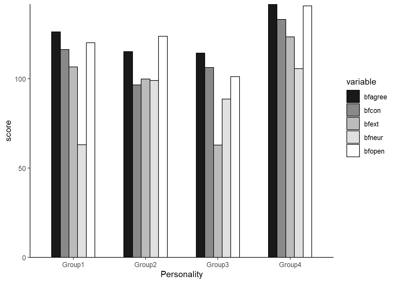

ggplot

ロジスティック回帰分析のグラフ

　なんかいい感じのグラフ描きたいなって思いますよね。
　ローデータがぶわーってプロットされてて、回帰直線・曲線がシューン！なってるやつ。
　下のコードを使います。　

library(ggplot2)
ggplot(data,                                                  　　#データを入れる
       aes(x=valiable1, y=as.numeric(categolical1)))+　　　　 　　#x軸とy軸の変数を決める
  geom_point(position=position_jitter(width=0.4,height=0.08), 　　
             alpha=.4,shape=21,size=1.5)+
    #ローデータをプロット。ただし、同じ箇所の点が重なってプロットされるので、散らす設定する
  stat_smooth(method="glm",
              method.args = list(family="binomial"(link="logit")))+  
    #ロジスティック曲線。ここはきちんと書かないとうまく表示されない。
  xlab("X軸の名前")+ylab("Y軸の名前")+    #x軸とy軸の名前を決める
  coord_cartesian(ylim=c(0,1))+　　　　　　　　　　#y軸の最小と最大の値を決める
  theme_classic()　　　　　　　　　　　　　　　　　#クラシックなデザインが好き

　すると、このようなものができます。

　　
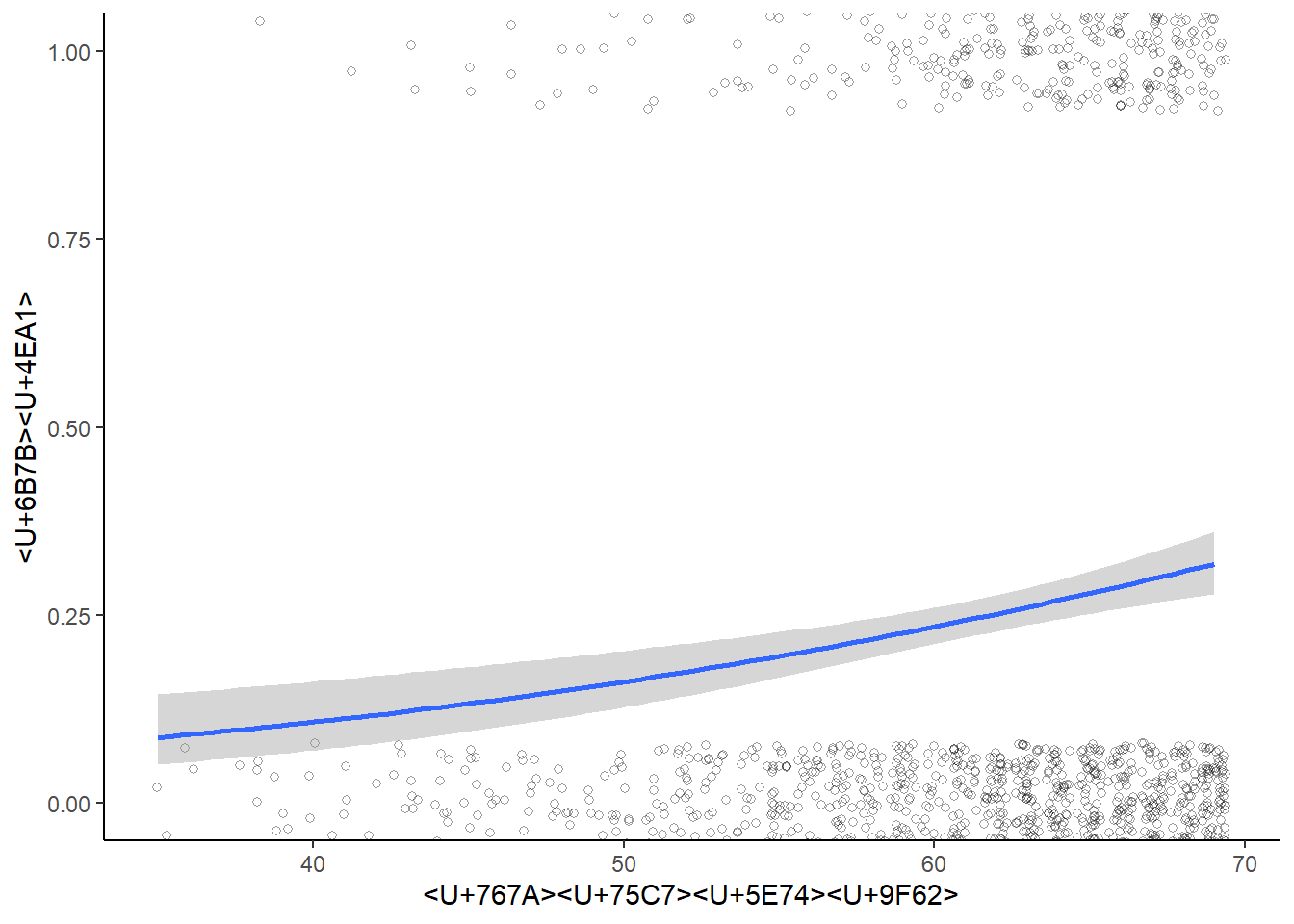
　なんか違うけど、データがそうならちゃんとS字になるはずなんだ・・・

軸の設定

ggplotでグラフを作成すると、x軸から棒グラフなんかが浮いてしまう（ラピュタ）。ラピュタを無くすならscale_y_continuous(expand = c(0,0))を加える
グラフの縦軸の指定は、たとえば０～１０にしたかったらcoord_cartesian(ylim=c(0,10))

Rmarkdown

yamlヘッダ

Rmarkdownでドキュメントを作るときの全体設定
改行やスペースが重要になるので注意
たとえば・・・

---
title: "Memo"
output: html_document:
  toc: true
  toc_float: true
---

　これだとエラーが出るし・・・

---
title: "Memo"
output: 
  html_document:
  toc: true
  toc_float: true
---

　これだとtoc: true以下が反映されない。

---
title: "Memo"
output: 
  html_document:        <- 改行
    toc: true           <- 半角2つスペースあける
    toc_float: true
---

　これでよし。