科学において測定は重要である。心理学においては、目に見えない心の働きを研究するうえで様々な質問項目が利用されてきており、それがお家芸にもなっている。複数からなる質問項目がいったいどのような概念を表しているのかは関心の高いところであるが、探索的因子分析は項目への回答に影響した因子の存在を統計的に抽出する手法である。
Rで分析する場合には以下のコードを用いる。
data <- XXX #分析したいデータを入れる

library(psych) #psychパッケージを使う

#因子数の決定
va<-data.frame(data$Q1,data$Q2,data$Q3,data$Q4,data$Q5,data$Q6,data$Q7,data$Q8,data$Q9,data$Q10,data$Q11) #因子分析にかける変数を取り出す

fa.parallel(va) #推定される最大の因子数(平行分析)
VSS(va,plot=FALSE) #推定される最小の因子数(最小平均偏相関)


#探索的因子分析
fa.result <- fa(va, nfactors = 4, fm = "minres", rotate = "promax") #たとえば因子数を4として、最小二乗法のプロマックス、どーん!
print(fa.result, sort = T, digit = 3, cut=0.3) #結果の表示。ソートかけて、桁数は3、0.3以下の結果はカット
上のコードでは、回転法はプロマックス回転、初期解の算出には最小二乗法を用いている。
回転法(rotate=)については直交回転と斜交回転を選択できる。直交回転なら“varimax”、斜交回転なら“promax”が使えるが、その他の回転法も直交回転と斜交回転のそれぞれ用意されている。
初期解の算出(fm=)には、最小二乗法なら“minres”、最尤法なら“ml”、主因子法なら“pa”が使える。他にもあり。
因子数の選定
因子分析をするにあたってはまず因子数の選定が必要になってくる。基本的には理論的な説明が可能であることが大切だろうが、統計的な算出方法もある。有名なのはスクリープロットでかくんとなってるところを基準に見るやつ。
その他、平行分析と最小平均偏相関という手法がある(どちらもpsychoパッケージに入ってる)。数学的なことはわからないけど、平行分析は因子数として選定され得る数を大きめに出す。一方、最小平均偏相関は因子数を倹約的に推定する。そのため、因子数はだいたい最小平均偏相関の値から平行分析の値までの間で分析していって、理論的な説明や因子分析のモデル適合度を見ながら最終的な因子数を決めるのが良さそう。
データセットとしてpsychパッケージに入っている“epi.bfi”を使用する。このデータセットにはアイゼンク性格検査(EPI)とBig 5尺度、ベック抑うつ性尺度、特性‐状態不安の得点が231人分入っている。
library(psych) #psychパッケージを使う

va<-epi.bfi #因子分析にかける変数を取り出す。ここではすべての変数を使う。- 平行分析
fa.parallel(va) #推定される最大の因子数(平行分析)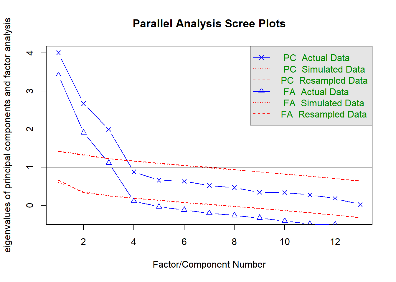
## Parallel analysis suggests that the number of factors = 3 and the number of components = 3- 最小平均偏相関
“The Velicer MAP achieves a minimum of 0.05 with…”のところのfactorsを見る。
VSS(va,plot=FALSE) #推定される最小の因子数(最小平均偏相関)##
## Very Simple Structure
## Call: vss(x = x, n = n, rotate = rotate, diagonal = diagonal, fm = fm,
## n.obs = n.obs, plot = plot, title = title, use = use, cor = cor)
## VSS complexity 1 achieves a maximimum of 0.73 with 3 factors
## VSS complexity 2 achieves a maximimum of 0.86 with 3 factors
##
## The Velicer MAP achieves a minimum of 0.05 with 3 factors
## BIC achieves a minimum of -22.79 with 6 factors
## Sample Size adjusted BIC achieves a minimum of -3.74 with 8 factors
##
## Statistics by number of factors
## vss1 vss2 map dof chisq prob sqresid fit RMSEA BIC SABIC complex
## 1 0.53 0.00 0.098 65 1253.38 2.0e-219 14.0 0.53 0.286 900 1105.6 1.0
## 2 0.70 0.76 0.076 53 704.54 1.2e-114 7.0 0.76 0.235 416 584.1 1.1
## 3 0.73 0.86 0.050 42 354.38 4.8e-51 3.1 0.90 0.183 126 258.9 1.3
## 4 0.71 0.86 0.065 32 262.74 4.6e-38 2.5 0.92 0.181 89 190.0 1.5
## 5 0.65 0.84 0.088 23 142.11 3.8e-19 2.1 0.93 0.153 17 89.8 1.7
## 6 0.63 0.85 0.116 15 58.85 4.0e-07 1.8 0.94 0.116 -23 24.8 1.7
## 7 0.66 0.83 0.147 8 21.71 5.5e-03 1.7 0.94 0.089 -22 3.5 1.8
## 8 0.65 0.81 0.218 2 0.81 6.7e-01 1.3 0.96 0.000 -10 -3.7 1.7
## eChisq SRMR eCRMS eBIC
## 1 1.5e+03 0.20267 0.222 1126
## 2 4.9e+02 0.11719 0.142 206
## 3 5.6e+01 0.03932 0.054 -173
## 4 2.8e+01 0.02811 0.044 -146
## 5 1.4e+01 0.01940 0.036 -112
## 6 3.3e+00 0.00952 0.022 -78
## 7 7.7e-01 0.00461 0.014 -43
## 8 1.5e-02 0.00065 0.004 -11探索的因子分析
因子数は3因子が良さそう。
fa.result <- fa(va, nfactors = 3, fm = "minres", rotate = "promax") #因子数を3として、最小二乗法のプロマックス、どーん!
print(fa.result, sort = T, digit = 3, cut=0.3) #結果の表示。ソートかけて、桁数は3、0.3以下の結果はカット
## Factor Analysis using method = minres
## Call: fa(r = va, nfactors = 3, rotate = "promax", fm = "minres")
##
## Warning: A Heywood case was detected.
## Standardized loadings (pattern matrix) based upon correlation matrix
## item MR1 MR2 MR3 h2 u2 com
## epiNeur 5 0.828 0.663 0.3371 1.05
## traitanx 12 0.825 0.821 0.1793 1.15
## bfneur 9 0.821 0.334 0.643 0.3566 1.33
## bdi 11 0.718 0.534 0.4663 1.01
## stateanx 13 0.662 0.451 0.5487 1.01
## epilie 4 0.187 0.8125 2.39
## epiE 1 1.015 1.050 -0.0497 1.02
## epiImp 3 0.757 0.568 0.4319 1.07
## epiS 2 0.702 0.584 0.4165 1.20
## bfagree 6 0.646 0.449 0.5512 1.03
## bfopen 10 0.642 0.404 0.5963 1.23
## bfcon 7 0.639 0.464 0.5359 1.35
## bfext 8 0.481 0.613 0.685 0.3155 1.90
##
## MR1 MR2 MR3
## SS loadings 3.127 2.541 1.834
## Proportion Var 0.241 0.195 0.141
## Cumulative Var 0.241 0.436 0.577
## Proportion Explained 0.417 0.339 0.244
## Cumulative Proportion 0.417 0.756 1.000
##
## With factor correlations of
## MR1 MR2 MR3
## MR1 1.000 -0.010 -0.257
## MR2 -0.010 1.000 0.117
## MR3 -0.257 0.117 1.000
##
## Mean item complexity = 1.3
## Test of the hypothesis that 3 factors are sufficient.
##
## The degrees of freedom for the null model are 78 and the objective function was 8.247 with Chi Square of 1854.125
## The degrees of freedom for the model are 42 and the objective function was 1.59
##
## The root mean square of the residuals (RMSR) is 0.039
## The df corrected root mean square of the residuals is 0.054
##
## The harmonic number of observations is 231 with the empirical chi square 55.713 with prob < 0.0764
## The total number of observations was 231 with Likelihood Chi Square = 354.378 with prob < 4.81e-51
##
## Tucker Lewis Index of factoring reliability = 0.6703
## RMSEA index = 0.1831 and the 90 % confidence intervals are 0.1628 0.1973
## BIC = 125.797
## Fit based upon off diagonal values = 0.985